Introduction
This is the first blog post in the series of the conspectus of the "Introduction to TLA+" course by Leslie Lamport. It would directly follows the course structure and would be a good reference for those who are taking the course because it adds some more additional information and explanations to the course material. So all credits are to Leslie Lamport and his course that can be found on his [website][1].
is based on temporal logic, so you may read about it in the [LTL and CTL Applications for Smart Contracts Security][2] blog post.
Inroduction to
is a language for high-level (design level, above the code) systems (modules, algorithms, etc.) modelling and consists of the following components:
- TLC — the model checker;
- TLAPS — the proof system;
- Toolbox — the IDE.
system is used to model critical parts of digital systems, abstracting away less-critical parts and lower-level implementation details. was designed for designing concurrent and distributed systems in order to help find and correct design errors that are hard to find by testing and before writing any single line of code.
OpenComRTOS is a commercial network-centric, real-time operating system [[3]] that heavily used during the design and development process and shared their experience in the freely available book [[4]]. And showed that using design gratefully reduce the code base size and number of errors and boost the engineering view overall.
Consequently, provides programmers and engineers a new way of thinking that makes them better programmers and engineers even when are not useful. forces engineers to think more abstractly.
Abstraction — the process of removing irrelevant details and the most important part of engineering. Without them, we cannot design and understand small systems. {.note}
An example of using in a huge company for verifying a system that many of us use daily is Amazon Web Services. They use to verify the correctness of their distributed algorithms and AWS system design [[5]]. The problem of algorithms and communication in distributed systems is well described in Leslie Lamport's paper "Time, Clocks, and the Ordering of Events in a Distributed System" [[6]].
A system design is expressed in a formal way called specification.
Specification — the precise high-level model. {.note}
defines the specification, but it cannot produce the code. But it helps come with much clearer architecture and write more precise, accurate, in some cases compact code. It is able to check properties that express conditions on an individual execution (a system satisfies a property if and only if every single execution satisfies it).
The underlying abstraction of is as follows: an execution of a system is represented as a sequence of discrete steps, where a step is the change from one state to the next one:
- discrete — continuous evolution is a sequence of discrete events (computer is a discrete events-based system);
- sequence — a concurrent system can be simulated with a sequential program;
- step — a state change;
- state — an assignment of values to variables.
Behavior — a sequence of states. {.note}
A state machine in the context of system is described by:
- all possible initial states – [what the variables are] and [their possible initial values];
- what next states can follow any given state – a relation between their values in the current state and their possible values in the next state;
- halts if there is no possible next state.
Control state — the next to be executed statement. {.note}
State machines eliminate low-level implementation details, and is a language to describe state machines.
State Machines in
uses ordinary, simple math. Consider a defined state machine example for the following C code
int i;
void main()
{
	i = someNumber();
	i = i + 1;
}
In order to turn this code into the state machine definition we need to pack the execution flow of this code into states (sets of variables). For the given example, it is obvious how to define i variable. But we also need to instantiate the control state. We call it a pc such as:
pc = "start"=i = someNumber();pc = "middle"=i = i + 1;pc = "done"= execution is finished.
Assume for this example someNumber() returns an integer from the [0:1000] interval.
To define the system we need to define the initial state of the system the the next possible system state, expressed as a formula, that can be reached from the current state.
Here is the formula of the C code above, not the sequence of execution.
- Initial-state formula:
(i = 0) /\ (pc = "start") - Next-state formula:
\/    /\ pc = "start"
      /\ i' \in 0..1000
      /\ pc' = "middle"
\/    /\ pc = "middle"
      /\ i' = i + 1
      /\ pc' = "done"
Since this is the formula, it respects such formulas properties as commutativity, associativity, etc.
Sub-formulas can also be extracted into their own definitions to make a spec more compact.
A == /\ pc = "start"
     /\ i' \in 0..1000
     /\ pc' = "middle"

B == /\ pc = "middle"
     /\ i' = i + 1
     /\ pc' = "done"

Next == A \/ B
From this spec, we see that there are two possible next states that can be reached beginning from the initial state. A states the beginning of the execution, assigning a number to i and moving to the next pc state equals p', B states the increment of i and moving to the final state.
Resources and tools
There are not many learning resources of ; however, there are some that we need to mention:
- Learning TLA+ — a portal with useful links;
- TLA+ toolbox binaries — a
Javabased IDE; - pdflatex — a required component to render
pdf;
Model Checking
Now, let us talk about TLC and model-checking related topics.
TLC computes all possible behaviors allowed by the spec. More precisely, TLC checks a model of the specification. {.note}
- TLC reports deadlock if execution stopped when it was not supposed to;
- TLC reports termination if execution stopped when it was supposed to.
allows writing theorems and formal proofs of those theorems.
TLAPS (TLA proof system) is a tool for checking those proofs, it can check proofs of correctness of algorithms.
Practically, the term spec (a specification) means:
- the set of modules, including imported modules consists of
.tlafiles; - the
TLAformula specifies the set of allowed behaviors of the system or algorithm being specified.
A specification may contain multiple models. The model tells TLC what it should do. Here are the parts of the model that must be explicitly chosen:
- what the behavior spec is (The behavior spec is the formula or pair of formulas that describe the possible behaviors of the system or algorithm you want to check);
- what TLC should check;
- what values to substitute for constant parameters.
Behavior spec
There are two ways to write the behavior spec:
- Init and Next
- A pair of formulas that specify the initial state and the next-state relation, respectively.
- Single formula
- A single temporal formula of the form , where
- is the initial predicate;
- is the next-state relation;
- is the tuple of variables;
- and is an optional fairness formula.
- A single temporal formula of the form , where
The only way to write a behavior spec that includes fairness is with a temporal formula, otherwise a spec would not have variables and in this case, TLC will check assumptions and evaluate a constant expression.
There are three kinds of properties of the behavior spec that TLC can check:
- Deadlock — A deadlock is said to occur in a state for which the next-state relation allows no successor states;
- Invariants — a state predicate that is true of all reachable states--that is, states that can occur in a behavior allowed by the behavior spec;
- Properties — TLC can check if the behavior spec satisfies (implies) a temporal property, which is expressed as a temporal-logic formula.
Model
The most basic part of a model is a set of assignments of values to declared constants.
Ordinary assignment
It is possible to set the value of the constant to any constant expression that contains only symbols defined in the spec. The expression can even include declared constants, as long as the value assigned to a constant does not depend on that constant (escape circular dependencies). A model must specify the values of all declared constants.
Model value
A model value is an unspecified value that TLC considers to be unequal to any value that you can express in . You can substitute the set of three model values for . If by mistake you write an expression like where the value of is a process, TLC will report an error when it tries to evaluate that expression because it knows that a process is a model value and thus not a number. An important reason for substituting a set of model values for is to let TLC take advantage of symmetry.
Example:
NotANat == CHOOSE n : n \notin NatIt defines
NotANatto be an arbitrary value that is not a natural number. TLC cannot evaluate this definition because it cannot evaluate the unboundedCHOOSEexpression. To allow TLC to handle the spec, you need to substitute a model value forNotANat. The best model value to substitute for it is one namedNotANat. This is done by the Definition Override. The Toolbox creates the appropriate entry in that section when it creates a model if it finds a definition having the precise syntax above or the syntax:NotANat == CHOOSE n: ~(n \in Nat), whereNatcan be any expression, andNotANatandncan be any identifiers.
Model values can be typed as follows: a model value has type T if and only if its name begins with the two characters T_ .
A model value declared in the model can be used as an ordinary value in any expression that is part of the model's specification.
Symmetry
Consider a specification of a memory system containing a declared constant Val that represents the set of possible values of a memory register. The set Val of values is probably a symmetry set for the memory system's behavior specification, meaning that permuting the elements in the set of values does not change whether or not a behavior satisfies that behavior spec. TLC can take advantage of this to speed up its checking. Suppose we substitute a set {v1, v2, v3} of model values for Val. We can use the Symmetry set option to declare this set of model values to be a symmetry set of the behavior spec. This will reduce the number of reachable states that TLC has to examine by up to 3!, or 6.
You can declare more than one set of model values to be a symmetry set. However, the union of all the symmetry sets cannot contain two typed model values with different types.
TLC does not check if a set you declare to be a symmetry set really is one. If you declare a set to be a symmetry set and it isn't, then TLC can fail to find an error that it otherwise would find. An expression is symmetric for a set S if and only if interchanging any two values of S does not change the value of the expression. The expression {{v1, v2}, {v1, v3}, {v2, v3}} is symmetric for the set {v1, v2, v3} — for example, interchanging v1 and v3 in this expression produces {{v3, v2}, {v3, v1}, {v2, v1}}, which is equal to the original expression. You should declare a set S of model values to be a symmetry set only if the specification and all properties you are checking are symmetric for S after the substitutions for constants and defined operators specified by the model are made. For example, you should not declare {v1, v2, v3} to be a symmetry set if the model substitutes v1 for some constant. The only operator that can produce a non-symmetric expression when applied to a symmetric expression is CHOOSE. For example, the expression CHOOSE x \in {v1, v2, v3} : TRUE is not symmetric for {v1, v2, v3}.
Symmetry sets should not be used when checking liveness properties. Doing so can make TLC fail to find errors, or to report nonexistent errors. {.danger}
Die Hard
Die Hard is an action movie from 1988. In this movie, there is a scene where are heroes need to solve a problem with two jugs in order to disable a bomb. The problem is to measure 4 gallons of water using 3 and 5-gallon jugs.
For the plot, search: "Die Hard Jugs problem" on YouTube or simply click here 🙂. We will solve this problem using .
First, we need to write the behavior. Let values of and represent a number of gallons in each jug.
Filling a jug is a single step; there are no intermediate steps.
Real specifications are written to eliminate some kinds of errors. {.tip}
has no type declarations; however it important to define a formula that asserts type correctness. It helps to understand the spec and TLC can check types by checking if such a formula is always .
TypeOK == /\ small \in 0..3
          /\ big   \in 0..5
Here, we define that small is an integer in the range [0:3] and big is an integer in the range [0:5]. But this definition is not a part of the spec.
The Initial-State Formula Init == small = 0 /\ big = 0 defines the initial state of the system.
The Next-State Formula defines possible transfers from state to state and is usually written as , where each formula allows a different kind of step.
Our problem has 3 kinds of steps:
- fill a jug;
- empty a jug;
- pour from one jug into the other.
We define the spec as follows:
Next == \/ FillSmall  \* fill the small jug
        \/ FillBig    \* fill the big jug
        \/ EmptySmall \* empty the small jug
        \/ EmptyBig   \* empty the big jug
        \/ SmallToBig \* pour water from small jug in the big jug
        \/ BigToSmall \* pour water from the big jug in the small jug
The names of definitions (like
FillSmall, etc.) must be defined before the usage (precede the definition ofNext). {.important}
FillSmall == /\ small' = 3
             /\ big' = big
When defining formulas we need to keep in mind thinking of the system as a whole and about steps as a transition from one state to another. In our case, it means that we cannot define FillSmall as FillSmall == small' = 3 because this formula doesn't have a part defining the second part of the program state (big). In another words, this formula turns if small' equals 3 and big' equals whatever. But this is not correct. In fact, if we fill the small jug, we keep the big jug in the state it is without changes.
Now, we define SmallToBig. There are two possible cases we need to consider:
SmallToBig == /\ IF big + small <= 5
                  THEN /* There is room -> empty small.
                  ELSE /* There is no room -> fill big.
SmallToBig == /\ IF big + small <= 5
                  THEN /\ big' = big + small
                       /\ small' = 0
                  ELSE /\ big' = 5
                       /\ small' = small - (5 - big)
VARIABLES small, big
TypeOK == /\ small \in 0..3 /\ big \in 0..5
Init == /\ big = 0 /\ small = 0
FillSmall == /\ small' = 3 /\ big' = big
FillBig == /\ big' = 5 /\ small' = small
EmptySmall == /\ small' = 0 /\ big' = big
EmptyBig == /\ big' = 0 /\ small' = small
SmallToBig == IF big + small =< 5 THEN /\ big' = big + small /\ small' = 0 ELSE /\ big' = 5 /\ small' = small - (5 - big)
BigToSmall == IF big + small =< 3 THEN /\ big' = 0 /\ small' = big + small ELSE /\ big' = big - (3 - small) /\ small' = 3
Next == / FillSmall / FillBig / EmptySmall / EmptyBig / SmallToBig / BigToSmall
=============================================================================
</DetailTag>
<br/>
If we create and run a model for this spec we will see no errors and this is fine; however, it doesn't check any particular invariant of our spec.
> Invariant is a formula that is $true$ in every reachable state.
{.note}
We have defined a `TypeOK` as a type definition for `small` and `big`, so we can add this formula as an invariant to check that this invariant is not broken.
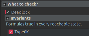
If we run it now, we still see no errors meaning `small` and `big` respecting their types in every reachable state.
Now we can solve the _die hard_ problem of pouring `big` with exactly 4 gallons of water. To do it, we add a new invariant `big /= 4` into the invariants section.
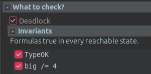
Here, this invariant works as a counterexample. An invariant is a formula that turns to $true$ in **every** reachable state. We need to find a state (actually a state sequence) where `big = 4`, so we negate this by the `/=` symbol that equals to $\neq$. With this new formula if we run the model, it finds an error (a state where an invariant is broken) and shows a sequence of states that led to this state.
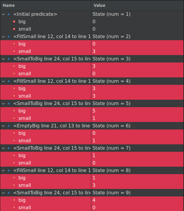
Now, we can see the exact steps that are required to be done to solve the problem and our heroes can move on.
## References
- [Leslie Lamport. Learning TLA+][1]
- [LTL and CTL Applications for Smart Contracts Security][2]
- [OpenComRTOS][3]
- [Eric Verhulst, Raymond T. Boute, José Miguel Faria, Bernhard H C Sputh, Vitaliy Mezhuyev. Formal Development of a Network-Centric RTOS. January 2011. DOI:10.1007/978-1-4419-9736-4. ISBN: 978-1-4419-9735-7][4]
- [Chris Newcombe, Tim Rath, Fan Zhang, Bogdan Munteanu, Marc Brooker and Michael Deardeuff.How Amazon Web Services uses formal methods. 2015, Communications of the ACM][5]
- [Leslie Lamport. Time, Clocks, and the Ordering of Events in a Distributed System. 1978. Massachusetts Computer Associates, Inc.][6]
[1]: https://lamport.azurewebsites.net/tla/learning.html
[2]: /blog/ltl-ctl-for-smart-contract-security/
[3]: https://en.wikipedia.org/wiki/OpenComRTOS
[4]: https://www.researchgate.net/publication/315385340_Formal_Development_of_a_Network-Centric_RTOS
[5]: https://www.amazon.science/publications/how-amazon-web-services-uses-formal-methods
[6]: https://amturing.acm.org/p558-lamport.pdf
<PostSocials type="blog" telegramId="14" />